Bias versus Variance, but what are they?

Why I'm writing this blog

Bias versus variance is a concept that is taught in the very first classes of machine learning. But I feel those classes leave a very superficial impression of the whole idea.

The problem goes deeper than that. Most students, I think, don't even know what bias and variance are to start with. Ask what the mathematical meaning of bias is, or of variance, and there is usually no answer beyond "bias is underfitting, variance is overfitting". Those are descriptions of what you see when things go wrong. They are not the definitions.

The definitions are actually short. For a model $\hat f$ trained on a random dataset $D$, and a test point $x_0$:

$$\text{Bias}(x_0) = \mathbb{E}_D\big[\hat f_D(x_0) - f(x_0)\big] = \mathbb{E}_D\big[\hat f_D(x_0)\big] - f(x_0)$$ $$\text{Var}(x_0) = \mathbb{E}_D\Big[\big(\hat f_D(x_0) - \mathbb{E}_D[\hat f_D(x_0)]\big)^2\Big]$$

Here $\hat f_D$ is the model trained on the dataset $D$, and $\mathbb{E}_D$ means an average over datasets: a fresh random dataset $D$ is drawn again and again, a model is trained on each one, and we average over all of those draws.

I'll derive where these come from at the end of this blog, so don't worry if the symbols look unfamiliar right now. The whole point of the story is that by the time we reach them, they will feel obvious.

What those first classes also don't teach is how this concept is stitched into the whole story of training a machine learning model. It isn't a side topic that sits next to training. It runs through all of it.

So I want to write the whole concept as a story, starting from the very beginning.

1. The pattern we want to learn

Let's start with something simple. Take a sine wave:

$$y = f(x) = \sin(x)$$

This is the pattern that exists in the world. It is the thing we want our model to learn. In real life we never get to see $f$. Here I'm going to keep it in my hands, because that is the only way to measure how far off a model is from the truth.

Now we try to get a dataset out of this pattern. A dataset doesn't come out as the clean function. Every observation comes with some noise, so what we actually get is:

$$y = f(x) + \epsilon$$

where $\epsilon$ is random noise, with mean zero and variance $\sigma^2$, drawn independently for every observation:

$$\mathbb{E}[\epsilon] = 0, \qquad \text{Var}(\epsilon) = \sigma^2$$

In a real problem we never get to see this noise distribution, so all we do is assume two things about it: that it averages out to zero, so the noise cancels over many draws and the pattern $f$ shows through, and that its spread is a fixed amount $\sigma^2$.

For all the experiments in this blog, I use $\sigma = 0.3$ (so $\sigma^2 = 0.09$), and each dataset has $n = 40$ points with $x$ picked uniformly from $[-3, 3]$.

2. Drawing the dataset more than once

Here is the part that is easy to miss.

When you train a neural network, the dataset feels like a fixed thing that was handed to you: a CSV, a folder of images, a table of measurements. But the way to think about it in this story is that it came out of exactly the process from the previous section. There is a pattern $f$, and the dataset you have is what that pattern produced once noise was added to every point: $y = f(x) + \epsilon$. It is not "the data". It is one draw.

And nothing special made it this draw. The same process could have handed you a different one, with different $x$ values and different noise on every point. Think of three people who each go out and collect their own dataset for the same problem. Below, the black curve is the true function $f(x) = \sin(x)$, and I drew a dataset from it three times:

• Red is the dataset I drew first.
• Yellow is the dataset I drew second.
• Green is the dataset I drew third.

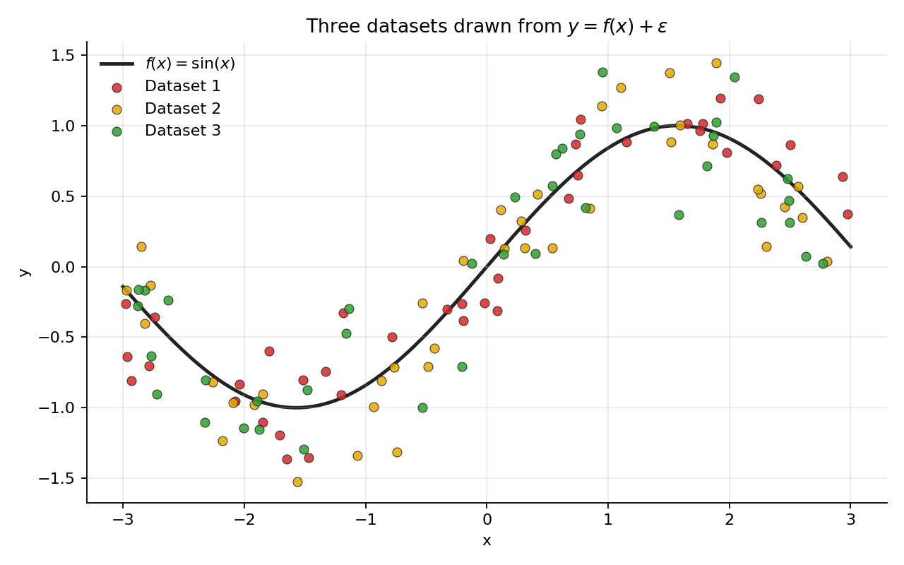Three datasets drawn from y = f(x) + epsilon

All three come from the same function, but the three draws came out different. The points sit at different places, and each one is pushed off the curve by a different amount of noise.

In practice you only ever get one of these. But keep all three in mind, because the entire idea of bias and variance lives in the gap between "the dataset I got" and "the datasets I could have got".

3. Training: fitting $\hat f$

We get a dataset $D = \{(x_i, y_i)\}_{i=1}^{n}$ and we want to recover $f$ from it. We can't, exactly, so we fit a model $\hat f$ as our best guess.

Two choices have to be made for training a model on data.

First, the model class. What family of functions are we allowed to pick from? I'll use polynomials of degree $d$:

$$\hat f(x) = w_0 + w_1 x + w_2 x^2 + \dots + w_d x^d$$

The degree $d$ is the complexity of the model. Degree 1 is a straight line, degree 3 is a cubic, and so on. A sine wave is not a polynomial, so no degree matches it exactly. The question is how close each one can get.

Second, the loss. How do we decide which function in the class is best? We take the one that does best on the training data, using squared error:

$$\hat f_D = \arg\min_{g \,\in\, \text{class}} \; \frac{1}{n}\sum_{i=1}^{n}\big(y_i - g(x_i)\big)^2$$

That is training. Notice the subscript $D$ on $\hat f_D$. The fitted model is a function of the dataset it was trained on. Give it a different dataset and you get a different $\hat f$.

Here is what that looks like. I trained three different models (degree 1, degree 3, and degree 8) on each of our three datasets. Each colour is the model trained on the dataset of the same colour.

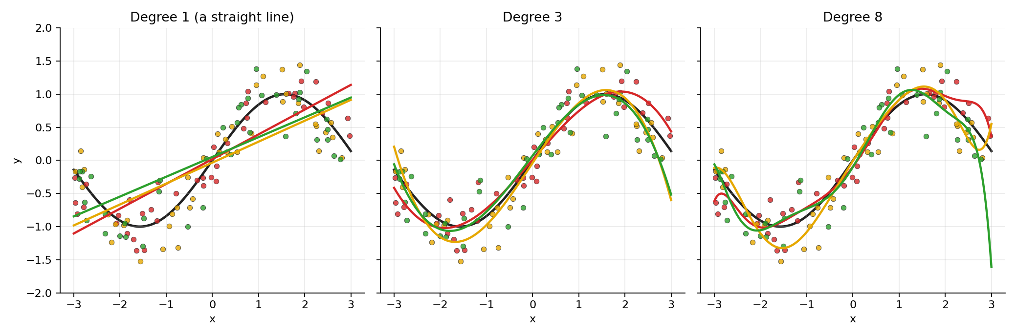Fits of degree 1, 2 and 8 on the three datasets

Bias and variance of each model, averaged over $x \in [-3, 3]$:

These are two different kinds of failure. The straight line fails because of what it is. The degree 8 polynomial fails because of what it got. Bias and variance are the names for these two.

To see them properly, imagine repeating the whole process: draw a fresh dataset, train the model, record the fit, and do it again and again. Now two separate questions can be asked about any model, at any point $x$.

Question 1: On average, where does the model land? Average all those fits and compare the average to the truth. For degree 1, the average fit is a straight line, while the truth is an S-shaped wave. They are far apart, even if we average over infinitely many datasets. That gap is the bias:

$$\text{Bias}(x_0) = \mathbb{E}_D\big[\hat f_D(x_0) - f(x_0)\big] = \mathbb{E}_D\big[\hat f_D(x_0)\big] - f(x_0)$$

For degree 3 and degree 8, the average sits close to the truth, so the bias is small. Both can bend the way a sine wave does, so on average they can find it.

Question 2: How much does the model move from dataset to dataset? Look at the spread of the fits around their own average. For degree 1 and 3 the spread is small. For degree 8 it is huge, especially near the edges. That spread is the variance:

$$\text{Var}(x) = \mathbb{E}_D\Big[\big(\hat f_D(x) - \mathbb{E}_D[\hat f_D(x)]\big)^2\Big]$$

It is simply the ordinary variance of the random number $\hat f_D(x)$, where the randomness comes from which dataset we happened to get.

So bias is how far the centre of the fits is from the truth, and variance is how wide the cloud of fits is around its own centre. That is all they are. How the numbers in the table above are calculated, and why these two in particular matter, is the next step: testing the model.

4. Testing: where the maths comes in

Training error is not what we care about. What we care about is how the model does on data it has never seen. So we take a fresh test point $x_0$, along with its label:

$$y_0 = f(x_0) + \epsilon_0$$

The test noise $\epsilon_0$ is fresh, so it is independent of the training set $D$ (and therefore of $\hat f_D$). It has $\mathbb{E}[\epsilon_0] = 0$ and $\text{Var}(\epsilon_0) = \sigma^2$.

The expected test error at $x_0$, averaged over everything random (which dataset we trained on, and the test noise), is:

$$\text{Err}(x_0) = \mathbb{E}_{D,\,\epsilon_0}\Big[\big(y_0 - \hat f_D(x_0)\big)^2\Big]$$

To keep the algebra readable, I'll write $f$ for $f(x_0)$, $\hat f$ for $\hat f_D(x_0)$, and $\bar f = \mathbb{E}_D[\hat f_D(x_0)]$ for the average prediction.

Step 1: separate the noise from the model

Substitute $y_0 = f + \epsilon_0$ and group the terms:

$$y_0 - \hat f = \epsilon_0 + (f - \hat f)$$

Square it:

$$(y_0 - \hat f)^2 = \epsilon_0^2 + 2\,\epsilon_0\,(f - \hat f) + (f - \hat f)^2$$

Take the expectation of each term.

• $\mathbb{E}[\epsilon_0^2] = \sigma^2$.
• The cross term is $2\,\mathbb{E}[\epsilon_0]\;\mathbb{E}[f - \hat f] = 0$, because $\epsilon_0$ is independent of $\hat f$ and has mean zero.

So:

$$\text{Err}(x_0) = \sigma^2 + \mathbb{E}_D\big[(f - \hat f)^2\big]$$

The first part, $\sigma^2$, is the noise in the test label. No model can predict it, because it was never in the pattern. It is the irreducible error.

Step 2: separate the model's error into two parts

Now we deal with $\mathbb{E}_D[(f - \hat f)^2]$. The trick is to add and subtract the average prediction $\bar f$:

$$f - \hat f = (f - \bar f) + (\bar f - \hat f)$$

Square it:

$$(f - \hat f)^2 = (f - \bar f)^2 + 2\,(f - \bar f)(\bar f - \hat f) + (\bar f - \hat f)^2$$

Take the expectation over $D$. Here $f$ and $\bar f$ are just fixed numbers (they don't depend on $D$), so $(f - \bar f)$ is a constant. And by the definition of $\bar f$:

$$\mathbb{E}_D[\bar f - \hat f] = \bar f - \mathbb{E}_D[\hat f] = 0$$

So the cross term disappears:

$$\mathbb{E}_D\big[(f - \hat f)^2\big] = \underbrace{(f - \bar f)^2}_{\text{Bias}^2} + \underbrace{\mathbb{E}_D\big[(\hat f - \bar f)^2\big]}_{\text{Variance}}$$

The first term is the squared gap between the average prediction and the truth, which is exactly the $\text{Bias}^2$ from the previous section. The second is the spread of $\hat f$ around its own average, which is exactly the variance. They did not come from nowhere. They fall out of the algebra.

The result

Putting both steps together:

$$\boxed{\;\text{Err}(x_0) \;=\; \text{Bias}(x_0)^2 \;+\; \text{Var}(x_0) \;+\; \sigma^2\;}$$

The error on unseen data splits into three parts:

1. Bias²: the model is systematically wrong, because the model class cannot represent the truth.
2. Variance: the model is unstable, because it changes a lot with the dataset it was trained on.
3. Noise σ²: the part nobody can fix.

Only the first two depend on our choice of model. That is why they are the ones we talk about.

5. Checking it numerically

A derivation is more convincing when you can watch it hold. Here is the decomposition measured from the 4000 datasets, at one test point $x_0 = 2$, where the truth is $f(2) = \sin(2) \approx 0.91$ and $\sigma^2 = 0.09$.

For each dataset I trained the model, predicted at $x_0$, and compared against a fresh noisy label $y_0$. The last column is the directly measured test error. The column before it is what the formula predicts.

The two right-hand columns agree to within sampling noise. The degree 1 model pays more in bias than in variance, because it cannot bend. The degree 3 model pays very little beyond the noise floor of 0.09.

The degree 8 model looks fine at $x_0 = 2$, with a variance of only 0.025. That is a good reminder that bias and variance are functions of $x$, not single numbers. If I average over the whole range $x \in [-3, 3]$, where the edges are very unstable for degree 8, the picture changes:

Over the whole range, degree 8 has by far the worst variance, and the formula still matches the measured test error.

Notice also the last column. The degree 8 model has the lowest training error of the three (0.069), and the worst test error (0.708). Training error only tells you how well the model fit the dataset it saw. It cannot see the variance.

6. Sweeping the complexity

Now I'll repeat the whole experiment for every degree from 1 to 8, averaging over $x \in [-3, 3]$, and plot where the test error comes from.

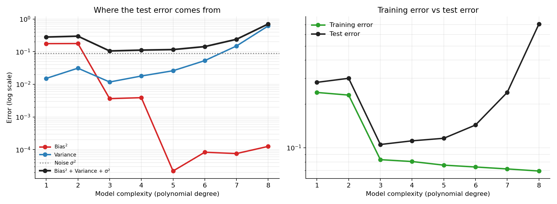Bias, variance and noise by model complexity; training and test error by model complexity

Reading the left panel (log scale, so every gridline is a factor of ten):

• Bias² (red) stays high for degrees 1 and 2 (a parabola is no better than a line at following a sine wave over a symmetric range), collapses at degree 3, and is tiny from degree 5 on. (Values around $10^{-4}$ or below are simulation noise.)
• Variance (blue) climbs as the model gets more flexible, apart from a small dip at degree 3 (the $x^2$ term in degree 2 has nothing to fit in an odd function like sine, so it only adds noise). More parameters means more ways to bend toward the noise of whichever dataset you got.
• Noise (dotted) doesn't care about the model at all. It is a floor.
• Total (black) is the sum of the three, and it is lowest at degree 3.

On the right panel, the training error keeps falling as the model gets more complex, while the test error goes the other way after degree 3. This is the gap that bias and variance explain. Training error rewards a flexible model for fitting its own dataset, and variance is the price it pays on every dataset that is not that one.

7. What I take away from this

The thing I wanted from this blog is a different way to see the concept. When we train a model, we are not really holding "a model". We are holding one sample out of a distribution of models, and that distribution exists because the dataset itself was one random draw out of many possible ones.

• Bias is about the centre of that distribution: if I could average over every dataset I might have got, would I land on the truth?
• Variance is about its width: how much does what I get depend on the luck of the draw?
• Noise is the part that was never in the pattern.

And the equation $\text{Err} = \text{Bias}^2 + \text{Var} + \sigma^2$ is not a rule someone made up for a nice picture. It is a three-line piece of algebra: add and subtract the right term twice, and use the fact that the cross terms have zero mean.

A few caveats worth keeping in mind:

• This clean split is for squared error. Other losses decompose differently.
• In my experiment I know $f$, so I can compute bias exactly. On real data you never do, which is why bias and variance are mostly ways of thinking about a model rather than numbers you read off a dashboard.
• Here the story ends with a neat U-shaped trade-off, but the real world is messier. For example, very large models trained in modern ways don't always follow this shape. That is a story for another blog.

All plots and numbers in this blog come from simulation.py: 4000 datasets, $n=40$, $\sigma=0.3$, polynomial least squares, seeds fixed.

References

• Goodfellow, Bengio and Courville, Deep Learning, Chapter 5: 5.4 Estimators, Bias and Variance